
텐서플로우 자격증 준비를 위한 공부를 하려고 합니다.
시험 문제 유형은 아래와 같으며 coursera와 udacity 강의를 보고 준비하려고 합니다.
-
Category 1: Basic / Simple model
-
Category 2: Model from learning dataset
-
Category 3: Convolutional Neural Network with real-world image dataset
-
Category 4: NLP Text Classification with real-world text dataset
-
Category 5: Sequence Model with real-world numeric dataset
www.udacity.com/course/intro-to-tensorflow-for-deep-learning--ud187
Intro to TensorFlow for Deep Learning | Udacity Free Courses
Developed by Google and Udacity, this course teaches a practical approach to deep learning for software developers.
www.udacity.com
www.coursera.org/learn/introduction-tensorflow/home/welcome
Coursera | Online Courses & Credentials From Top Educators. Join for Free | Coursera
Learn online and earn valuable credentials from top universities like Yale, Michigan, Stanford, and leading companies like Google and IBM. Join Coursera for free and transform your career with degrees, certificates, Specializations, & MOOCs in data science
www.coursera.org
Category 5: Sequence Model with real-world numeric dataset
필요한 라이브러리들을 import합니다.
import tensorflow as tf
import numpy as np
import matplotlib.pyplot as plt
import csv
!wget --no-check-certificate \
https://storage.googleapis.com/laurencemoroney-blog.appspot.com/Sunspots.csv \
-O /tmp/sunspots.csvdef plot_series(time, series, format="-", start=0, end=None): plt.plot(time[start:end], series[start:end], format) plt.xlabel("Time") plt.ylabel("Value") plt.grid(True)sunspots 데이터를 불러온 다음에 데이터를 확인해보겠습니다.
time_step = []
sunspots = []

with open('/tmp/sunspots.csv') as csvfile:
  reader = csv.reader(csvfile, delimiter=',')
  next(reader)
  for row in reader:
    sunspots.append(float(row[2]))
    time_step.append(int(row[0]))

series = np.array(sunspots)
time = np.array(time_step)
plt.figure(figsize=(10, 6))
plot_series(time, series)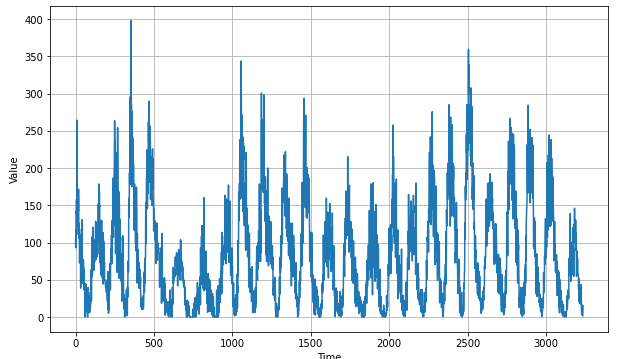
trian과 valid 데이터 셋을 만들어 줍니다.
split_time = 3000
time_train = time[:split_time]
x_train = series[:split_time]
time_valid = time[split_time:]
x_valid = series[split_time:]
window_size = 30
batch_size = 32
shuffle_buffer_size = 1000windowed_dataset은 Time Series 데이터셋을 생성할때 매우 유용합니다.
window : 그룹화 할 윈도우의 크기(갯수)
drop_remainder : 남은 부분을 버릴지 살릴지
shift : 1 iteration 당 몇 개씩 이동할 것인지
flat_map : 데이터셋에 함수를 apply 해주고 결과를 flatten하게 펼쳐 줍니다.
shuffle : 데이터 셋을 섞어 줍니다.
def windowed_dataset(series, window_size, batch_size, shuffle_buffer):
    series = tf.expand_dims(series, axis=-1)
    ds = tf.data.Dataset.from_tensor_slices(series)
    ds = ds.window(window_size + 1, shift=1, drop_remainder=True)
    ds = ds.flat_map(lambda w: w.batch(window_size + 1))
    ds = ds.shuffle(shuffle_buffer)
    ds = ds.map(lambda w: (w[:-1], w[1:]))
    return ds.batch(batch_size).prefetch(1)
window_dataset을 이용해서 time series 데이터셋을 생성해줍니다.
train_set = windowed_dataset(x_train, window_size, batch_size, shuffle_buffer_size)
print(train_set)
print(x_train.shape)
LSTM 모델을 생성해줍니다.
model = tf.keras.models.Sequential([
                                    tf.keras.layers.Conv1D(filters=32, kernel_size=5,strides=1, padding="causal",activation="relu",input_shape=[None, 1]),
                                    tf.keras.layers.LSTM(64, return_sequences=True),
                                    tf.keras.layers.LSTM(64, return_sequences=True),
                                    tf.keras.layers.Dense(30, activation="relu"),
                                    tf.keras.layers.Dense(10, activation="relu"),
                                    tf.keras.layers.Dense(1)])

model.summary()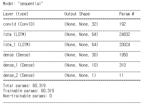
LearningRateScheduler : 모델 학습동안에 일반적으로 행하는 것은 epochs에 따라 learning rate를 decay시켜주는 것입니다.
옵티마이저는 Stochastic Gradient Descent로 확률적 경사 하강법을 사용하였습니다.한번 학습할 때 모든 데이터에 대해 가중치를 조절하는 것이 아니라, 램덤하게 추출한 일부 데이터에 대해 가중치를 조절합니다.
lr_schedule = tf.keras.callbacks.LearningRateScheduler(lambda epoch: 1e-8 * 10 ** (epoch / 20))
optimizer = tf.keras.optimizers.SGD(lr=1e-8, momentum=0.9)
model.compile(loss=tf.keras.losses.Huber(),
              optimizer=optimizer,
              metrics=["mae"])

history = model.fit(train_set, epochs=100, callbacks=[lr_schedule])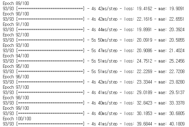
학습이 끝난뒤 예측해보겠습니다.
def model_forecast(model, series, window_size):
    ds = tf.data.Dataset.from_tensor_slices(series)
    ds = ds.window(window_size, shift=1, drop_remainder=True)
    ds = ds.flat_map(lambda w: w.batch(window_size))
    ds = ds.batch(32).prefetch(1)
    forecast = model.predict(ds)
    return forecast

rnn_forecast = model_forecast(model, series[..., np.newaxis], window_size)
rnn_forecast = rnn_forecast[split_time - window_size:-1, -1, 0]

plt.figure(figsize=(10, 6))
plot_series(time_valid, x_valid)
plot_series(time_valid, rnn_forecast)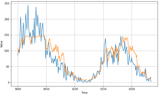
tf.keras.metrics.mean_absolute_error(x_valid, rnn_forecast).numpy()21.613613
'Data Analysis > Tensorflow' 카테고리의 다른 글
| [tensorflow] sarcasm (0) | 2021.01.03 |
|---|---|
| [tensorflow] horses_or_humans (2) | 2021.01.02 |
| [tensorflow] Fashion MNIST (0) | 2020.12.30 |
| [tensorflow] Basic / Simple model (0) | 2020.12.30 |
| [tensorflow] pycharm 설치 및 환경설정 (0) | 2020.12.18 |